BMS links with a Statistical Analysis package called Breeding View. This package is propriety software developed by VSNi and is based on Genstat and uses ASREML for mixed model analysis of plant breeding trials. Breeding View is designed to quickly perfor perform routine analysis for plant breeding. It is not so versitile versatile as a statistical package, such as the full version of Genstat, which is required for research analysis.
...
Breeding View is a stand alone program which must be downloaded to your windows 64 bit computer, and installed. Before you can use it you must sspply a license key by clicking Help>Activate license: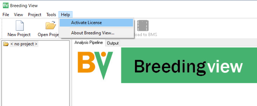
Once the license is activiated activated you can use Breeding View but it normally requires an internet connection to check the validity of the license before running. There is more informations information about installing and licensing Breeding View in the manual.
https://bmspro.io/1937/breeding-management-system-manual-40/install-breeding-view-statistical-application
...
From the STUDIES menu select Single-Site Analysis: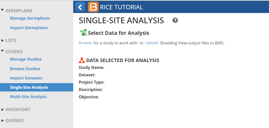
Browse for the study containing the data to be analysed. We will select the trial we created and imported in the previous tutorial – CGM20AVT for me. Highlight the file and click Select.
The Study will open and display the factors it contains: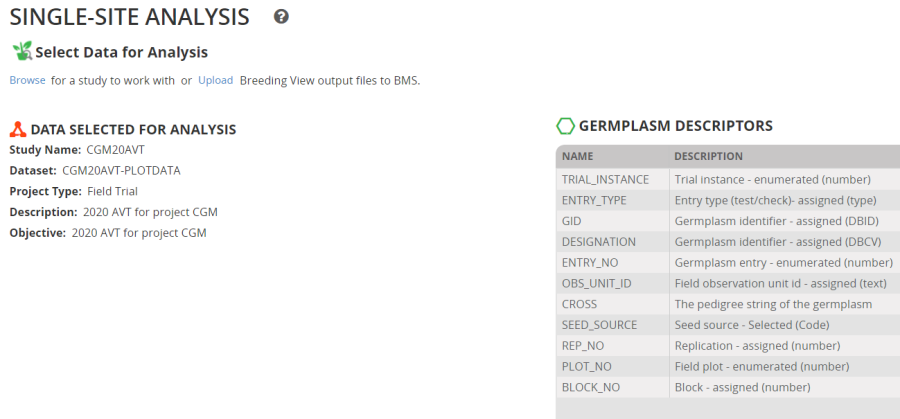
And the traits it contains: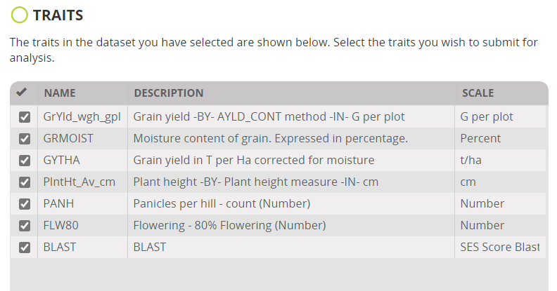
By default all the traits are selected for Analysis. Deselect those which do not require analysis, GrYld_wgh_gplant and GRMOIST in our example do not require analysis. We will analysis the BLAST score even though it is not a continuous variable, it is an ordinal variable with a fair number of classes.
Any of the non-analysed varaibles variables can be specified to be covariates in an analysis of covariance for the analysed variables. We will not specify any covariates. Click Next.
On the form to Specify Options for Breeding View Analysis you must first select the variable which distinguishes between sites. You always have the variable TRIAL_INSTANCE available, but usually the LOCATION_NAME is preferable. We will select LOCATION_NAME.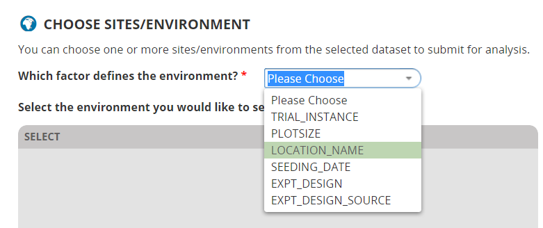
And we will select all the locations for analysis: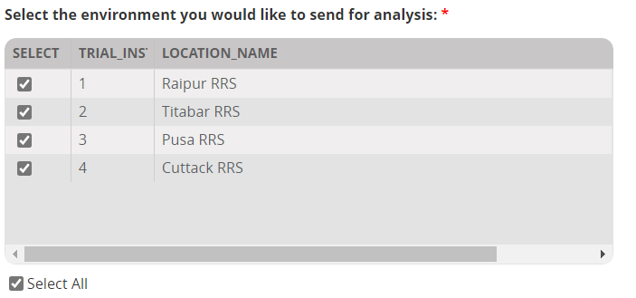
Next you must specify the design type. Since our design was imported the system doesn does not know the design type. Select Incomplete block design: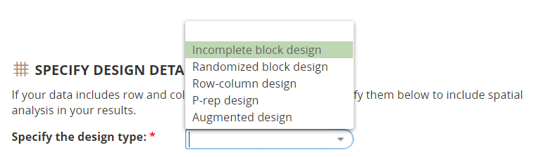
This selection opens a form requesting the design variables – Rep and Block for our design. REP_NO and BLOCK_NO have been selected by default. There are also fields for specifying variables indicating the row and column layout of the trial. These variable are created by the process of making and Field Plan (which you can do in the Study Manager using Actions>Field map options>Make a Fieldmap). If the row and column layout is available then Breeding View will attempt a Spatial Analysis of the trial to reduce the error variability. If they are not available (as in our case) or a spatial analysis is not wanted the variables should not be selected.
Finally you need to specify the variable which deines defines the entries in the trial. You always have ENTRY_NO available, but usually the DESIGNATION is preferred: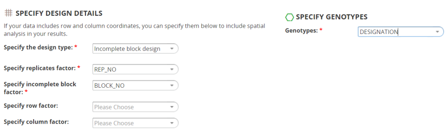
Once the analysis details are specified you must request a Download of the Input Files for Breeding View. Click Download Input Files:![]()
This will download a zip file with the names of the study.zip – CGM20AVT.zip for me.
You need to extract the files from this zip file int a directory where the analysis will be performed. There are two files in the zip, one csv file which contains the data to be analysed and on xml file which contains the instructions for the analysis.
...
Once the files have been extracted you can run Breeding View and clcik click the Open Project icon and navigate to the directory where the files have been extracted. Select the xml file and click Open.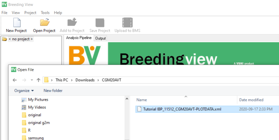
The Single Site Analysis Pipeline will be activiatedactivated: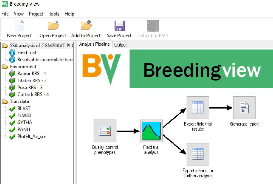
This contains a menu on the left showing the Environments and the Traits which have been specified for analysis. You can select or deselect any and all sites and or traits for analysis. We will leave all the sites and all the variables to be analysed.
The right hand panel shows the pipeline of tasks for single site analysis. Each task has a default configuration, but can also be specially configures by righright-clicking of the task icon and selecting settings and adjusting the menu.
For example right click on Quality control phenotypes, click Settings and you will get the following menu: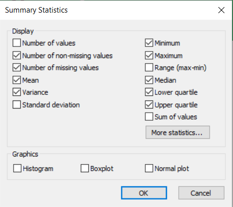
We will accept the default settings for this task. However right click on the icon for Generate Report and select settings: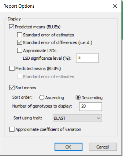
You will see that the table of means will be sorted on BLAST score in descending order and only the 20 entries with largest BLAST score will be printed in the report. This is clearly not what we want, so you should change the setting to 32 genotypes to be displayed and sort using GYTHA and we would also like to see the Coefficient of Variation so we check that box, then click OK.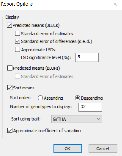
To run the analysis right click on the Quality crontol control phenotypes icon and select Run selected envirment environment pipeline.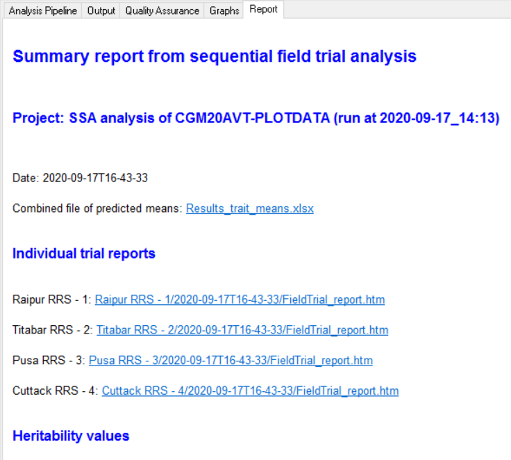
To understand how to interpret the Breeding View output you can colsult consult the Mamual Manual under the topic Statistical Analysis at this URL
https://bmspro.io/1823/breeding-management-system/tutorials/maize-single-site-analysis-4-location-batch
...
The output from the Single Site Analysis is stored in the folder where the original downloaded files were extracted. A folder has been added with the results for each site, and two other folders are added, one called combined with a table of means over all locations, and another called upload which contains a zip file of means ready for uploading to the BMS.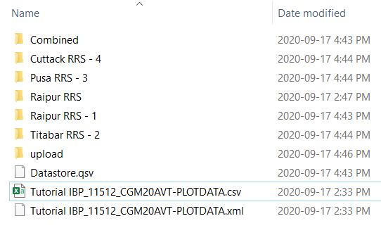
In the BMS click Single Site ANlsysis Analysis for the Statistical Analysis menu, then click upload to upload Breeding View output files.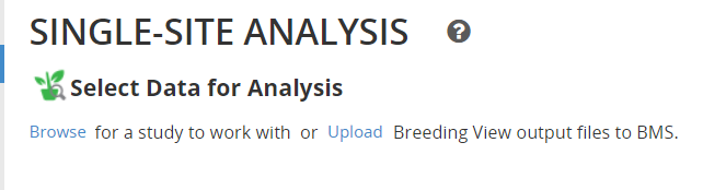
Select the study for which the analysis has been completed – CGM20AVT for me.
Click Browse and navigate to the Upload folder in the Breeding View output directory. Select the zip file from the upload folder.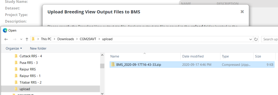
Click open and then upload. The upload will take a few seconds to complete and you should receive a Success notice.
To see the means in BMS you can use the Browse Studies app for the INFORMATION MANAGEMENT menu.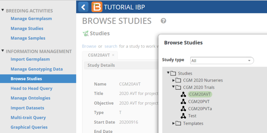
Open the study for which you wish to see the means, click on Datasets and select the means dataset: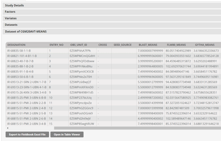
You can export any of the datasets from this application as well.
...
From the STUDIES menu select Multi-Site Analysis and browse to the study for which you have uploaded means and for which you wish to do a multi-site analysis. You need at least three sites for a GxE analysis and four or more is better. As with the single site anlaysis analysis you are asked to specify the variable defining sites – usually use LOCATION_NAME, and for genotypes – usually DESIGNATION. Next the form asks if your environments are already grouped in some way which would account for significant GxE interactions. Usually we do not know about groupings at the early stage, and mostly do not have enough environments for subsets.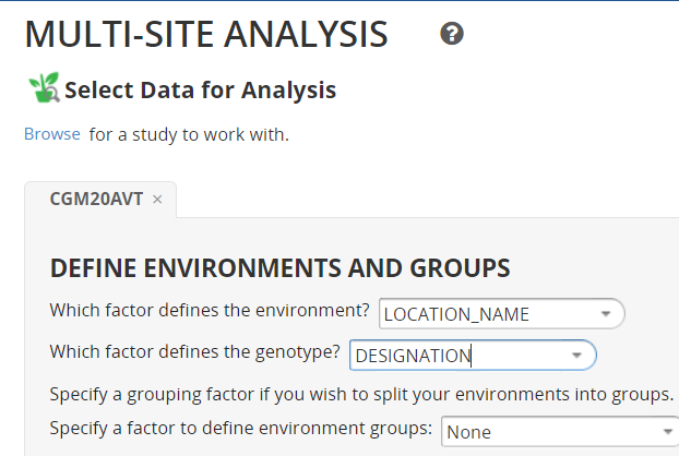
The form also show the variables in the study and asks the user to check the traits for which a GxE analysis is required. We will analysis only GYTHA. Click Next.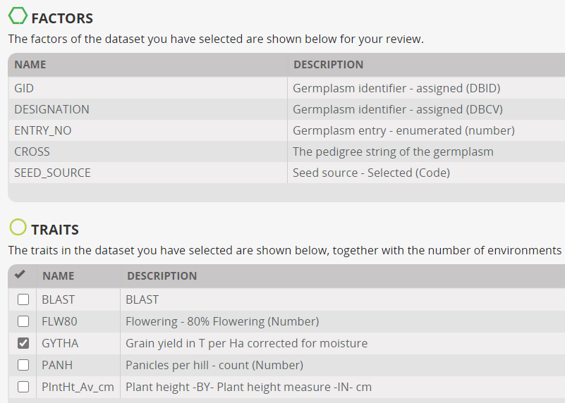
A form displaying a data summary for the locations and the selected traits is presented. This allows you to eliminate environments for which there is insufficient data of for which the heritability is too low, and similarly at the botton bottom you can eliminate traits. Whe We have already limited out traits to one, but we notice that Environment 2 has zero heritability. There would not normally be any reason to include an environment in a GxE alanysis which was showing a very small heritability so we will uncheck environment 2 and continue the analysis with just three environments.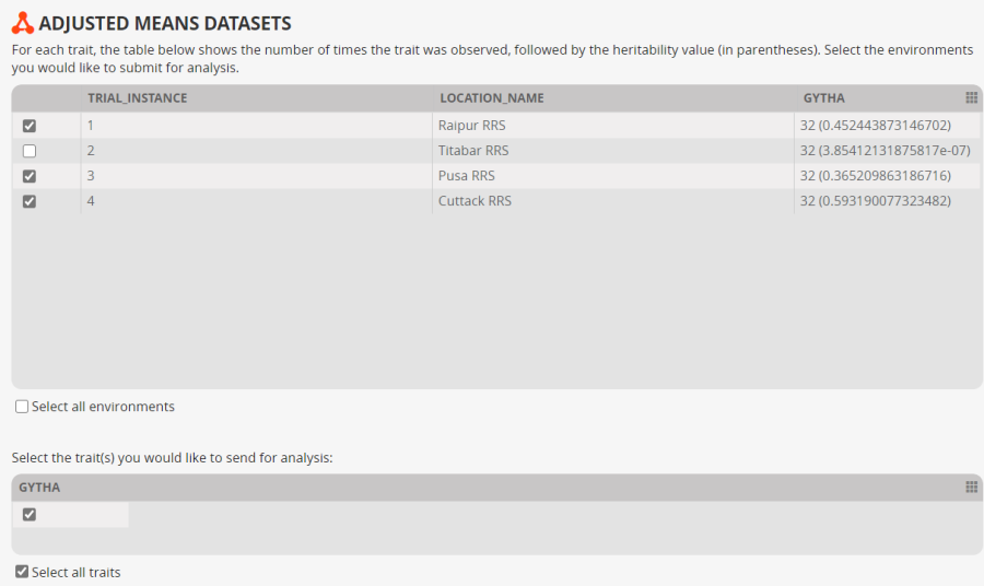
Click Download Input Files at the bottom of the form.
A zip file with the name of the study will be downloaded. You could extract the three files in this zip to a directory for analysis.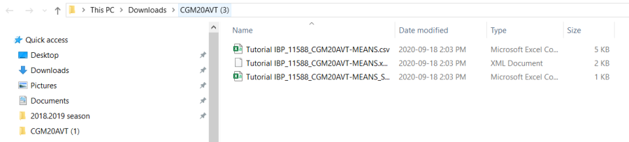
...